


Collocation methods for solving differential equations
"The easiest way to solve a differential equation is to know the answer in advance" - Feynman

Suppose you have a standard first order differential equation/initial value problem of the form
If you’re lucky the equation has a form that has known solutions, but often there’s no analytical solution, and we have to resort to numerical integration. This might take the form of an “Euler forward” solution like this:
Where you step through Δt times until your stopping point tf. Perhaps you use a Runge-Kutta method or some other algorithm, but basically you’re stepping through one time point at a time to get your solution.
Today I want to show you an altogether different method for numerically solving differential equations, one which solves the DE over your entire integration grid simultaneously, instead of one step at a time. Moreover, this method will return a solution which is a function of time, so you can query as many points as you like, as opposed to trying to make Δt ever smaller to get more points. This method has great advantages in optimization and optimal control when you need to optimize something subject to dynamic constraints. I won’t be covering how to do that in this post, but perhaps I can do so in a future post if there’s interest.
Collocation methods primer
The general idea with this method is to assume that the solution to your differential equation can be accurately represented by a polynomial
Here I’ve used what’s called a “monomial basis” to represent the polynomial, i.e. a linear combination of {1, x, x2, …} because it’s intuitive and easy to build off of, but there are other representations that can be used which will have different properties for numerical stability. I’ve also labelled our representation with a ~ to distinguish it from the “true” solution.
So we’ve “solved” our problem of trying to find a solution to the differential equation, but now we’ve introduced a new problem in that we have n+1 unknown coefficients. If t0 is 0, as is often the case, then we can trivially find a0, but a) that’s not always the case and, more importantly, b) we still have n unknown coefficients, and for the sake of keeping our solution general we might as well assume t0 ≠ 0.
So we need to come up with n+1 equations, where can we find them? Well, we can do this trick: since we have a “solution” to our DE, we can plug it back into the DE at n+1 points, and now we have a (generally nonlinear) system of n+1 equations! This set of points is known as the “collocation points”
Brief aside: why is it called collocation? Frankly I'm not sure. "co-location" make some amount of sense, since we're "co-locating" our solution and our DE at certain points, but to my knowledge the accepted pronunciation is more like "collo-cation" so ¯\_(ツ)_/¯tn can be tf but it doesn’t have to be. As you can see, once we’ve solved this system of equations we have a function x(t) and we can evaluate it wherever we like!
Some implementation
Let’s try implementing this in Python. We’ll start with the most basic of DE’s so that we can easily check our work
import numpy as np
from scipy.optimize import root
import matplotlib.pyplot as plt

# Set up our approximation functions and a function to generate the system of equations we'll need

def xtilde(t, a0_to_an):
    degree = len(a0_to_an) - 1
    terms = [a0_to_an[i] * t**i for i in range(degree+1)]
    return sum(terms)

def xtildedot(t, a0_to_an):
    degree = len(a0_to_an) - 1
    terms = [a0_to_an[i] * i * t**(i-1) for i in range(1, degree+1)]
    return sum(terms)

def create_system_of_eqns(dxdt, x0, t0, tf, degree):
    collocation_points = np.linspace(t0, tf, degree)
    def system(coeffs):
        eq_ic = [
            xtilde(t0, coeffs) - x0
        ]
        eq_points = [
            xtildedot(ti, coeffs) - dxdt(tf, xtilde(ti, coeffs))
            for ti in collocation_points
        ]
        return np.array(eq_ic + eq_points)
    return system

# And now we can set up the problem

def dxdt(t, x):
    return x

t0 = 0
x0 = 1
tf = 1

# It should be obvious that the solution to this DE is e^t

degree = 3
system = create_system_of_eqns(dxdt, x0, t0, tf, degree)
initial_guess = np.zeros(degree + 1)
solution = root(system, initial_guess)

# Finally we print out some information and plot our numerical solution as compared to the analytical one
if solution.success:
  print(f'Solution converged in {solution.nfev} function evaluations')
else:
  print(f"Solution failed to converge: {solution.message}")
plt.plot(t:=np.linspace(t0, tf), np.exp(t), label="$e^t$")
plt.plot(t, xtilde(t, solution.x), label=r"$\tilde{x}$")
plt.grid()
plt.legend()
plt.show()

You can see from the plot that a simple 3rd order (cubic) polynomial fits et quite well on this small interval. And since our result is a function of time, it’s quite easy to use the quadrature tools in scipy to integrate the absolute value of the error as compared to the analytical solution over this time range, but we’ll leave this as an exercise for the reader.
A more challenging application
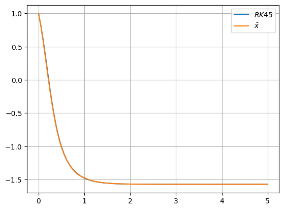
Let’s see how this works on a more challenging differential equation. We’ll try to apply it to ẋ = -(x+5)cos(x) over [0, 5] with an initial value of 1. The solution converges for polynomials of high enough order, but it’s not a very good solution.

A visual inspection of the “true” solution (provided by standard numerical integration with RK45) reveals that it’s probably hopeless to try to model this entire domain with a single polynomial. In particular the nearly flat section from ~2 to 5 needs a much lower order polynomial than the more dynamic section before then.
Fortunately it’s quite easy to extend this concept of collocation with the notion of a piecewise polynomial solution.
Of course, now we need (n+1)*m equations, but this is not difficult. We can select n collocation points for each segment, and start each segment with a condition that it must be equal to the end of the previous segment, in order to preserve continuity.

The image above shows what this might look like for two elements each representing a polynomial of degree 2, for which we need 3 equations each.
Obviously there’s a lot of “bookkeeping” involved in trying to keep straight all of our collocation points and polynomials and polynomial coefficients. I would encourage you to try modifying the above code on your own to take all this into account, as going through the bookkeeping yourself can help to illuminate and solidify these concepts. For those who want to check their code against a solution you can find it here.
With all of this implemented we can return to our DE from above. After some experimentation we find that using 5 elements each with degree 7 gives us a very good fit.
An inspection of the coefficients will show that for the elements after t~2 the coefficients of the higher order terms are very small. In theory we could have different degree polynomials for different elements, but we don’t necessarily know ahead of time which degree to use for which section, and this would add a considerable amount of bookkeeping overhead, particularly as we refine our grid.
Conclusion
Now that we know we can solve differentiation equations with this method, we must ask the question, should we? Of course the answer depends on the application. If you just want to integrate a DE once for a quick experiment, standard numerical techniques like RK45 are probably sufficient.
Where this technique has the potential to really shine is when the DE is being solved in a loop, perhaps in some kind of iterative optimization where the solution to the DE needs to be recomputed on every iteration. Careful setup of a collocation method can significantly improve the performance of such a method, particularly since you can use the coefficients from a previous iteration as an initial guess for the coefficients of the current iteration.
And besides the scenario above, it never hurts to have a few extra tools in your toolbox. You never know when you might need them!
Exercises
For these exercises, use ẋ = sin(x) over [0, 5] with an initial value of 1. Using the single element code above will be sufficient.
Try the code above and replace dxdt with np.sin(x), and replace the analytical solution either with numerical integration or find an analytical solution. Can you get the collocation approach to converge for *any* order polynomial?
What if you change the initial guess from `np.zeros` to `np.ones`. Can you find a degree for which the solution converges?
Now turn your attention to the collocation points. We have a uniform grid, but collocation of often done on grid points that are the roots of orthogonal polynomials. Trying using `roots_legendre` from `scipy.special` to come up with collocation points. Those roots are in the domain [-1, 1] so you’ll need to scale them. How does this improve the solution? Does combining it with a better initial guess produce an even better estimate?
For a real challenge, try implementing Lagrange interpolating polynomials as a basis, instead of the monomial basis. They require a little more work to implement because they are intricately linked with the collocation points, unlike the monomial basis. However the coefficients of the Lagrange polynomials are the values of the state itself at the collocation points, which can make it easier to come up with an initial guess for those coefficients.